Author Archives: RainerUnwin

Collations and text scan efficiency

SQL anti-patterns are an often misunderstood concept. One very basic anti-pattern is a leading wildcard character in a textual search. It can have really bad effects on a large table and yet there are always instances of it becoming a requirement. You see this all too often especially when reporting style queries are run on a transactional database. Lets say that for some reason we wanted to find all of our customers whose surnames end in “ith” like Smith for instance. We might write a query like the one below: –

[code language=”sql”]
SELECT FirstName, LastName, DOB
FROM dbo.table1
WHERE col1 LIKE LastName ‘%ith’;
[/code]

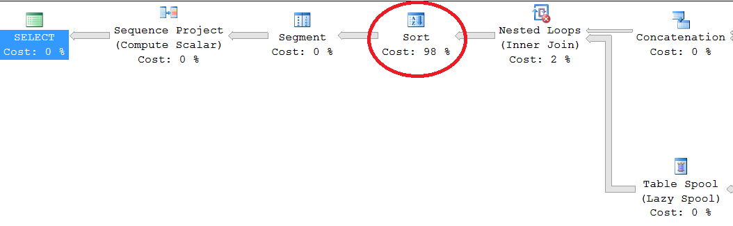
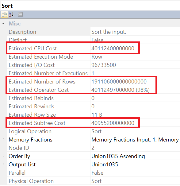
Even if we have an index on LastName the best we can do is to scan the index. An index in SQL Server, much like an index in a phone directory, is of little help to us here. If you were to try and find every surname in a phone book that ended with “ith” you’d have to read every entry in the index. Ok that’s still better than looking at every page in the phonebook. Although our query requests 3 columns which may not be in the index and therefore the lookups to the actual data may actually make the index scan and lookup slower than a scan of the entire data.

Anyway onto something quite trivial that can speed up such a query. If the term collation in this posts title jumped out at you as a potential performance improvement then you’re correct. Of course we could also use a full text index but that carries overhead and all sorts of other joys. Lets assume that either this isn’t a common query or you’re low on disk space and full text indexes are not an option just for this post. I might cover those in another post at some other point. A collation is a way of ordering something in our case the text that we are storing and the way that SQL Server can use different collations affects the query above. Let’s look at an example, it’s quite a long script so I’d suggest you copy and paste it and then read along after: –

[code language=”sql”]
SET NOCOUNT ON;
GO

IF OBJECT_ID( N’tempdb..#results’, ‘U’ ) IS NOT NULL DROP TABLE #results;
GO
CREATE TABLE #results( duration INT, run VARCHAR(30) );

— Create a test DB
USE [master];
GO
IF( SELECT DATABASEPROPERTYEX(N’TestDB’, ‘Collation’) ) IS NOT NULL DROP DATABASE TestDB;
GO

CREATE DATABASE [TestDB]
ON  PRIMARY
( NAME = N’TestDB’, FILENAME = N’C:\SQLData\DataFiles\TestDB.mdf’ , SIZE = 20480KB , FILEGROWTH = 20480KB )
LOG ON
( NAME = N’TestDB_log’, FILENAME = N’C:\SQLData\LogFiles\TestDB_log.ldf’ , SIZE = 20480KB , FILEGROWTH = 20480KB )
GO

USE [TestDB];
GO

— Create and populate a relation
IF OBJECT_ID( N’dbo.LoadsOfData’, ‘U’ ) IS NOT NULL DROP TABLE dbo.LoadsOfData;
GO
CREATE TABLE dbo.LoadsOfData(
id INT IDENTITY PRIMARY KEY CLUSTERED
, filler CHAR(200) NOT NULL DEFAULT ‘a’ COLLATE SQL_LATIN1_GENERAL_CP1_CI_AS — Notice the normal collation
);
GO

WITH n( n ) AS(
SELECT 1 UNION ALL SELECT 1 UNION ALL SELECT 1 UNION ALL SELECT 1 UNION ALL SELECT 1 UNION ALL
SELECT 1 UNION ALL SELECT 1 UNION ALL SELECT 1 UNION ALL SELECT 1 UNION ALL SELECT 1
), vals( n ) AS (
SELECT ROW_NUMBER() OVER( ORDER BY n.n ) – 1
FROM n, n n1, n n2, n n3, n n4, n n5
)
INSERT INTO dbo.LoadsOfData( filler )
SELECT REPLICATE( CHAR( 48 + n % 10 ) + CHAR( 65 + n % 26 ) + CHAR( 97 + (n + 1) % 26 ) +
CHAR( 48 + (n + 3) % 10 ) + CHAR( 65 + (n + 5) % 26 ) + CHAR( 97 + (n + 7) % 26 )
, 30 )
FROM vals;
GO

— Time something that will scan
DECLARE @start DATETIME2( 7 ) = SYSDATETIME(), @a INT;

SELECT @a = COUNT(*)
FROM dbo.LoadsOfData
WHERE filler LIKE ‘%e%’;

SELECT @a = DATEDIFF( mcs, @start, SYSDATETIME() );

INSERT INTO #results( duration, run ) VALUES( @a, ‘With normal collation’ );
GO

— Change the collation
ALTER TABLE dbo.LoadsOfData ALTER COLUMN filler CHAR(200) COLLATE LATIN1_GENERAL_BIN; — Now make the column a binary collation
GO

— Try again
DECLARE @start DATETIME2( 7 ) = SYSDATETIME(), @a INT;

SELECT @a = COUNT(*)
FROM dbo.LoadsOfData
WHERE filler LIKE ‘%e%’;

SELECT @a = DATEDIFF( mcs, @start, SYSDATETIME() );

INSERT INTO #results( duration, run ) VALUES( @a, ‘With binary collation’ );
GO

— Yes the applied selects are inefficint but they take less space 🙂
SELECT duration, run
FROM #results
UNION ALL
SELECT (select duration from #results where run like ‘%normal%’) / (select duration from #results where run like ‘%binary%’), ‘Improvement multiple’;
[/code]

So lets go over what we’re doing for clarity.

  1. First we drop and then create a test database to use, always good to clean up
  2. We create a temp table to hold the results
  3. Create a table to use and populate some nonsensical test data
  4. Now we run our wildcard query and get the execution time. Note that we don’t return any results to the client so this is basically the execution as best as we can get it. We get the duration in microseconds
  5. Then we change the column to use a binary collation
  6. Now we re-run our test in the same way as before and again store the results in our temp table
  7. Finally we get the durations and a difference from the results table. I don’t care about the inefficiency here 🙂

As you can see, even with this small table there is a remarkable difference in duration and we see an improvement of about 15 times. This is better than I was expecting, I was expecting nearer 8 times which is more usual but the point is well made by the difference. Also in this case we didn’t have an index on the text column but because that is by far the majority of the data anyway it wouldn’t make that much difference.

Generating a sequential number list on the fly

I have often found a need to generate a sequential number list for a query, or at least that it would make the solution easier. This post looks at a way of achieving this. We’ll start with the premise that we need to generate a sequential number list starting from a specific number and of specific length. As a result of this assertion we need to be able to pass in these parameters.

The easiest way to solve this problem is to store a list of numbers in a table. This is surely simple and effective, the main drawback being we don’t know the numbers we’re going to need up front. If we use bigints anywhere in our code base we might need to cover off the entire range which means storing bigints from min to max. That would require a lot of storage space and may not be feasible. We will therefore look at another method. The main point being that I wish to generate these numbers on the fly. This in itself presents an issue which I will mention at the end of this post.

Lets start with something simple like the query below and build on it: –

[code language=”sql”]
select row_number() over(order by a.object_id)
from sys.all_columns a;
[/code]

This generates a fairly simple plan that is also very efficient. However unless we already have a huge number of columns this is severely limited in the size of result set returned. We can of course use a cross join back to the same DMV again to generate a larger list. This works however may not encompass the entire range we want (ie, not enough numbers generated) and there are more issues if we join this DMV more than twice. Let’s take a look at what happens. If we cross join this DMV twice or more (Four times here – please note that I am only using commas for brevity here, this is considered bad practice and doesn’t make it into my production code) then we start to see a sort operator in the execution plan: –

[code language=”sql”]
select row_number() over(order by a.object_id)
from sys.all_columns a,
sys.all_columns b,
sys.all_columns c,
sys.all_columns d,
sys.all_columns e;
[/code]

Sort operator on multi cross join

This sort operator presents a problem. A sort is a blocking operation which means that it must complete before we can return the result set to the next operator in the plan. Looking at the properties of this operator we can see that life is too short to wait for this complete.

Sort operator for multi corss join

We need to get rid of this operator, so lets play a simple trick on the opitmizer and make our lives a little easier. Rather than return a sorted list at this stage lets return all one’s. The optimizer is a pretty clever cookie a lot of the time and will realise that this won’t need to be sorted, a 1 cannot be determined to go before or after another 1 and be sorted. The downside is we don’t get our sequential numbers but that is a trivial problem to solve. So we have the below query (Which I won’t run, nor do I recommend it to you because the result set is massive).

[code language=”sql”]
select 1
from sys.all_columns a,
sys.all_columns b,
sys.all_columns c,
sys.all_columns d,
sys.all_columns e;
[/code]

Now we have removed the sort operator and we have a massive range of numbers to return. We’re most of the way there. Here is the new plan without the sort: –

No sort returning all ones

Ok the estimated cost is still huge and we’ve only got a massive list a one’s but lets solve both of those issues next. The great thing that we achieved by removing the sort operator is that we no longer have any blocking operators in our query plan. We can prove this by running the query. The select starts to return rows immediately, once you’ve confirmed this cancel the query because it takes too long to run and will most likely exceed execution memory. This is the case because when the query executes the select asks the next operator (The compute scalar) for a row to be returned. The compute scalar asks the loop join and so on and so forth until we get to the operators that are getting the rows. None of these operators block so the select is free to start returning rows as soon as we start the query. We can easily limit the result set with a top operator and we can get our number list back with the use of the row_number() function. To do so we just need to wrap the current result set returning it as a derived table. That would look like the below and we now have a query we can execute: –

[code language=”sql”]
select top (100000)
row_number() over(order by dt.i) as seq_no
from (
select 1
from sys.all_columns a,
sys.all_columns b,
sys.all_columns c,
sys.all_columns d,
sys.all_columns e
) dt (i);
[/code]

The plan that we get is also a lot nicer however because it’s of a decent size I suggest you look it over on your own computers. Now in this case I have used a specific top quantity but again this is trivial to sort. Lets create a function that gives us total flexibility here, also we’ll move the top operator for another slight efficiency gain: –

[code language=”sql”]
create function dbo.consecutive_numbers (
@top bigint
, @offset bigint
)
returns table
as
return
select row_number() over(order by v.i) + (@offset – 1) as number
from (
select top (@top) 1
from sys.all_columns a,
sys.all_columns b,
sys.all_columns c,
sys.all_columns d
) v (i);
[/code]

If we create this function, in say a “tools” database, we can then call it at any time to generate a numbers list. We can specify the required start point and the limit to be returned. Also because cross joining sys.all_columns 4 times generates a huge result set it is unlikely that we will exhaust the list of numbers we can generate. At any rate it’s far less likely than it is to exhaust our patience waiting for the result set to be returned. So if you don’t want to store a table to get at consecutive numbers then this might be a possible solution for you. I hope that this brief look at the optimizer proves useful to anyone looking for a solution to a similar problem. My final solution is presented below, it is almost identical but uses two inline table valued functions just because of the increased flexibility. Also I use just two cross joins because I wrote this for an OLTP environment. In case anyone is interested I did a speed run to compare the two variants and they were identical and only ever got to 33% CPU on my Surface Pro 3 so this is not hugely CPU intensive.

[code language=”sql”]
if object_id(N’dbo.many’) is not null drop function dbo.many;
go
create function dbo.many (
@top bigint
)
returns table
as
return
select top (@top) 1 as number
from sys.all_columns a,
sys.all_columns b,
sys.all_columns c;
go

if object_id(N’dbo.cons_nos’) is not null drop function dbo.cons_nos;
go
create function dbo.cons_nos (
@top bigint
, @offset bigint
)
returns table
as
return
select row_number() over(order by number) + (@offset – 1) as number
from dbo.many(@top)
go;
[/code]

If you have tried running the solution presented in this post you will most likely realised that there is a limitation with this solution. The size of the result set requested has a profound effect on performance. If you request a very large result set (Say over 100,000,000 records) then you might be waiting a while for the list to return, even on a high end modern server. In any case large result sets will always cost time so this is no different. However storing the required values ahead of time may prove a quicker solution which you should test if you need all the performance you can get.

Using OPTIMIZE FOR to affect plan operators

This is a post about an interesting plan change I noticed while experimenting having attended a presentation by Adam Machanic (Blog) at sqlbits. For anyone who doesn’t know who Adam is I suggest finding any videos of his previous PASS sessions, he is a very clever chap who deals with some unique problems giving him amazing insights into the optimizer. Adam was at sqlbits in the UK, great conference which I highly recommend by the way, talking about row goals. Once that the session is available online I would recommend people watch it. Truly great session about helping the optimizer choose the correct plan without forcing a fragile plan using “hints”. Incidentally this isn’t how I generate my sequential number lists at present, please see this post for my current solution.

If you’ve read my other posts you may have noticed that I don’t do as much development as DBA work. Maybe my posts don’t necessarily bear that out though. In any case I like developing T-SQL and I like to focus on efficiency where I can. There is no reason to leave performance to randomness and we should, in my opinion, attempt to guide the optimiser down the right path in how we write our queries. Now as most of you will know we can “Hint” (Better called force) certain plans with hints. However we can use hints in more subtle ways and this is where I came across a nice plan change while playing with what I learnt from Adam. I have used simpler queries below for illustration. First off the query was based on the below, this gave me the flexibility to change any part of the record set I wanted to as well as the expected row counts (I used SQL Server 2014): –

[code language=”sql”]
declare @i int = 20
, @j int = 20
, @k int = 20;

select row_number() over(order by c.i)
from (
select top (@i)
[object_id]
from sys.all_columns
) c (i)
cross join (
select top (@j)
[object_id]
from sys.all_columns
) d (i)
cross join (
select top (@k)
[object_id]
from sys.all_columns
) e (i);
[/code]

Ordinarily I would not be using the top statements or sub-queries because this is just a nice way to generate a number list (In this case 1 – 8,000). However I put this in a while loop to run 1,000 times to do some performance checking on it. I didn’t run the exact same query because I didn’t want inserts to be the main bottleneck however this query better illustrates what I want to show. The execution time on my Surface Pro 3 was about 5.2 seconds. The plan had a nasty little sort operator in it. I wondered if I could make this disappear.

row_goals_with_sort

I changed the script to the below (After some playing around with some optimize for values) and got a rather nice improvement in both the plan and the run time. The latter was down to 1 second.

[code language=”sql”]
declare @i int = 20
, @j int = 20
, @k int = 20;

select row_number() over(order by c.i)
from (
select top (@i)
[object_id]
from sys.all_columns
) c (i)
cross join (
select top (@j)
[object_id]
from sys.all_columns
) d (i)
cross join (
select top (@k)
[object_id]
from sys.all_columns
) e (i)
option (optimize for (@i = 40, @j = 30, @k = 30));
[/code]

What struck me was that the first query had a 62MB memory grant and a rather expensive sort that didn’t exist when I hinted larger numbers. However the largest number hinted had to be the first (@i) and also had to exceed the others by a certain value. I tracked this performance improvement down to a merge concatenation as opposed to straight up concatenation. The later being more expensive because it sorts all the records not just the first join (Which is sufficient in this query).

row_goals_with_merge_concat

More impressively when I used larger numbers for the declared variables I still needed the hint to benefit from the plan shape I had generated, even when these were identical to the values I was passing in. Again I benefitted massively from not needing a sort space memory grant (Which due to memory limitations on my Surface rapidly spills to disk) and not needing the sort at all. On larger values this was very easily noticeable. The same 5x performance improvement was noticeable for almost any range of values in the declares. However to make them show I did need to use a loop, as described before, because generating 30,000 numbers is near instant. At 27,000,000 the runtime changed between 22 seconds and 4.5 seconds. Again the later was with the optimize for hint.

I would like to finish this post with another big thank you to Adam Machanic and what I learnt at SQLBits. I will be doing some more playing in this area and there may be some more posts to follow.

How much data does a differential backup need to backup

I recently wanted to know how much of my database a differential backup would actually need to read and backup. I soon had an idea to scan the Differential Change Map (DCM) pages in the data files. To understand what these pages track lets have a quick review of how SQL Server stores data.

How does SQL Server store data?

SQL Server stores data for each entity in database pages, pages are 8KB chunks of data in the data files. These pages are organised into 64KB extents, or 8 contiguous pages. SQL Server also stores allocation pages that track the usage of pages/extents within the data files. One of these allocation pages is the DCM which tracks whether or not any part of any page in an extent has been modified since the last full backup. So if I had a data page on the 30th page in my database and this was amended since the last full backup then the relevant DCM page would show that the 4th extent had been modified since the last full backup.

The theory

The DCM pages track changes to extents since the last full backup. This allows SQL Server to determine, very efficiently, which extents need to be backed up in the next differential backup. The first DCM page is the 7th page (zero based so page 6) in the database. The below command can be used to view the page: –

[code language=”sql”]
DBCC PAGE( myDatabase, 1, 6, 3 ) WITH TABLERESULTS, NO_INFOMSGS;
GO
[/code]

Also DCM pages are repeated every 511,232 pages in the database. Given this information we can use the below pseudo code as a basis for developing our script: –

  1. Get a list of all the data files (Exclude log files) in our database
  2. Iterate over all the data files to load all the DCM pages
    1. Follow all the DCM pages in each file
    2. Read all the data in those DCM pages
    3. Save the relevant data into a temp table
  3. Using the result table work out how many pages in each DCM interval, the section of a data file that the DCM relates to, will be backed up
  4. Sum the results
  5. Generate a summary result set

The results

I have a sample output in a couple of tables below as a summary of a scan against a small test database. I have previously run a very similar script successfully against a multi-terabyte database. Every DCM page represents just under 4GB of data in your database so even at 4TB you would have only about 1,000 DCM pages to read. There is obviously a small amount of overhead for the temp tables and to get the file list. Thereafter for every DCM page there will be 14 page reads. So as you can see this is a pretty light-weight script and highly efficient.

Summary result set

total_pagesaltered_pagespercent_changed
2816273697.16

Detailed output, this shows one result line per contiguous set of extents where at least one record in that extent has been modified

file_idstart_pageend_pagealtered_pages
1027362736

The script

In order to use this script please change the database name on line 60. Then run the script. I would recommend running against a test or dev instance initially. Lastly in preference to running against a production instance I personally run this against a log-shipped database. Please let me know if this script proves useful or if you have any issues.

DCM_scanner

Index Depth for Partitioned Tables

One really useful function that Microsoft provide with SQL Server is the INDEXPROPERTY function. With it you can get the depth of an index, which is the number of pages in the index that need to be read to get from the root to the leaf. Assuming a table called dbo.test with an index pk_test you could use a query like the one below: –

[code language=”sql”]
SELECT INDEXPROPERTY(OBJECT_ID(N’dbo.test’, N’U’), N’pk_test’, ‘IndexDepth’);
[/code]

The problem with this in-built function is that it doesn’t work on partitioned tables, yielding a not so helpful NULL as a result. Now of course there is a way to get the index depth for each balanced tree structure of each partition with sys.dm_db_index_physical_stats. My issue here is that I don’t want that much information and I want to know how much load I will be putting on the server. Load here being measure in terms of reads and by extension buffer pool usage. So I rolled my own script to look up the index depth of all partitions of an index. We’ll get to that in a moment, first I thought I’d explain why I cared.

I was looking at some indexes that someone else had created with the DTA (Database Tuning Advisor). A very nice feature that works quite well when used properly. Not so great when someone feels that a scatter gun tactic of throwing all recommended indexes at a database would be clever. One place where the DTA falls down is that it doesn’t know what you were trying to achieve with your design. As such the DTA may well recommend a great index that breaks something else for you. For example with partitioned tables you can lose the ability to fast switch if you have non-aligned indexes. Here’s an example of something similar to what I had. Lets assume you have 100 partitions each of depth 3 (Which we don’t yet know but my script can help you there). You have a primary key which is a nice surrogate integer identity, often recommended but not always advisable. The partitioning key is a datetime column. Finally you also have a non partition aligned index on the primary key alone, depth 4. The clustering key is on the identity however in practice you have to be in the right partition so effectively it might as well be datetime, id instead.

Now if I wanted to check the existence of a record by looking up the ID, for example, then the optimiser would in this situation correctly conclude that the non-aligned index is ideal. 4 reads and we’re done. If we used the clustering key we’d need to access each partition and check each one because we cannot get the datetime field first (we only have the ID). Well that’s going to be 300 reads. 3 reads per partition. Yep them 4 reads sure are looking good right about now. Now the downside here was that this non-aligned index would prevent me fast switching partitions. So yes it was ideal for the data access but it was really bad for my data purge. Picture a very upset DBA about this time 🙂

I now had some work to do to sort this out, but before I did that I came across the annoyance with INDEXPROPERTY so I made a stored proc to help. The proc can be created in any DB and can then be pointed at any other DB, so I recommend putting it in a Tools or DBA database if you choose to use it. By the way it uses dynamic SQL. I really like dynamic SQL for it’s power and flexibility. In the right hands dynamic SQL is a really powerful tool, but only in the right places. I’ve seen been some really bad performance issues in the past where dynamic SQL was the right way to go and no other way would have been nearly as good. In this case I needed dynamic SQL to easily let me construct the query to get the root pages of each partition. I also needed dynamic SQL to capture the root page data with DBCC PAGE. The proc will check for the existence of the database, which should be the only part that might allow SQL injection, and bails out if the database cannot be found. Also there is error handling for this and anything deemed serious will be logged. Otherwise you should get a result set. This script should work in SQL Server 2005+ although I cannot test it on all versions. Please let me know if you use it and find it useful or find any errors.

Get index depth for partitioned tables

Indirect Checkpoints in SQL Server prior to 2012

Just a short post this time. I was preparing a transaction log demo for my local user group the other day. For this I needed to load a bunch of data into my test database without the log growing. Unfortunately I was loading the data so fast that the log grew several times. Now I’m a somewhat impatient kind of guy so I wanted a solution where I could load the data at maximum speed. I ran a few scripts to diagnose the issue and it turns out that SQL Server wasn’t checkpointing my database often enough.

As you are most likely aware Microsoft helpfully gave us indirect checkpoints in SQL Server 2012. These may well have solved the issue for me. I could simply have configured my database to a much shorter recovery interval and the rate of checkpoints would have increased. Unfortunately I happened to be running SQL Server 2008 R2 on this test server which meant I couldn’t use that feature. Now I could equally well have created a simple job to repeatedly run checkpoints. However I wanted a more flexible solution to the problem.

I ended up writing a very basic and potentially helpful script that checks how much of the transaction log is currently active before it runs the next checkpoint. I then added a delay so I could run it in a tight loop and checkpoint just after the log is 50% full. I was using the simple recovery model so this relates quite closely to when the last checkpoint was run and allows the log to clear after the next checkpoint. The thing that caught me out was that I wrote the script on my 2014 instance and wanted to deploy it on my 2008 R2 instance. Turns out that Microsoft added an extra column to DBCC LOGINFO so I got an error. A quick amendment later and I was ready to test my script. One major point of note is that this will only work to keep the log from growing if you have short transactions and are running in the simple recovery model. However if you just wanted to reduce the time that it takes recovery to run then simply increasing the checkpoint rate will work. No need for anything like my script for that.

The script is below (Slight edit on December 7th 2014 for DBCC command I forgot about), although with the loop removed and ready to be run in a job where you can set the seconds between executions with the job interval

ManualIndirectCheckpoint

Plan Cache Pollution

I was working on a pretty common and simple problem the other day. I’m sure you’ve all seen servers where there are plenty of single use plans in the plan cache. All those single use plans are just using up memory for no real gain. One major point to bear in mind with all this is that SQL Server is basically an in memory system. SQL Server doesn’t directly update the data on disk. The data is loaded into memory, updated in memory and then eventually flushed to disk. This means that anything that consumes memory is taking away resources that may, or may not, be better utilized. Lets take a closer look, albeit still an overview at what happens with a read/write, and then solve our plan cache bloat problem.

Review of how SQL Server reads/updates data

As I already stated SQL Server will not update data directly on disk. Instead SQL Server will load the data from disk into memory. During ramp up (After a reboot or instance restart and before target memory is reached) the I/O is at the extent level (8 contiguous pages on disk) although can be more with read ahead during scans. Once that SQL Server has achieved steady state the I/O is at the “Right” size. What does right mean? Well if SQL Server needs an extent or more it will read that extent or read ahead for more data during that I/O. However if SQL Server needs a single 8KB page then the I/O operation is an 8KB page. This read is represented internally as a PAGEIOLATCH_XX (Where XX is usually EX or SH for write or read respectively) if you look in sys.dm_os_wait_stats. You can use the below query to see all in memory page latches: –

[code language=”sql”]
SELECT *
FROM sys.dm_os_wait_stats
WHERE wait_type LIKE N’pagelatch%’; /* Change to pageiolatch% to see the input/output latches which are similar except for I/O */
[/code]

With our data in memory, lets assume a single 8KB data page, SQL Server will now take the appropriate latch. Most likely either a PAGELATCH_SH (Read) or a PAGELATCH_EX (Write). We’ll ignore transactional locks and all other synchronisation mechanisms, they’re well covered elsewhere and not what I wanted to cover, also this is a simplification for this article. If we’re reading from the page SQL Server will now process that operation, likewise if writing or updating a record SQL Server has the opportunity to do so. This operation is now entirely in memory.

In the case of a write SQL Server will also generate a log record which will be flushed/hardened to disk on commit (Well that’s a good enough explanation for this post but isn’t always entirely accurate). The record would also be hardened to disk on rollback however another compensation log record would also be created and hardened to disk, so we would write 2 log records in case of a rollback. After, and only after, the log record of the changes have been flushed to disk can the data page be written out to disk. It is also important to appreciate that the write of the data page may not happen right away.

So when is a data page written to disk? There are several internal operations that can flush a data page to disk, sorry if a I miss something out here but they are basically as below (For checkpoint I have listed some operations that cause checkpoints): –

  • Checkpoint – this writes all dirty pages (Pages in memory that have data changes not yet reflected on disk) for a database to disk
    • Automatically based on the server or database recovery interval
    • Adding or removing a data or log file to/from a database
    • Any kind of backup operation
    • Any kind of clean shutdown of a database
    • Creating a database snapshot
    • Anything that causes a database snapshot to be created under the covers (eg, DBCC CHECKDB)
    • Putting a database into read only mode
    • Manual checkpoints
  • Lazywriter – this process tries to keep some free buffers (Think of these as memory slots for pages) in the buffer pool and will flush the least recently used pages to disk as needed
  • Eager writing – this process goes to work during operations like bulk loads and will flush those pages that are written to disk very quickly

So you can appreciate that allocating memory to execution plans that won’t be used more than once wastes memory that could be used for data. That is until SQL Server ages those plans out automatically. Also more data pages in the buffer pool means less physical I/O and therefore shorter waits. This generally leads to better performance. I say generally because I don’t want you to run off and flush your plan cache, that would be a very bad idea.

The solution

Now we can get back to the meat of this post. If you run the below query, which might be pretty intensive depending on your server spec so test first, you’ll see how many single use plans you have cached. These are execution plans that SQL Server needed to generate to execute a query but have not been used since that one time. I have grouped the results for single use plans into plans created in the last hour and older:-

[code language=”sql”]
SELECT SUM(CASE WHEN execution_count = 1 AND creation_time > DATEADD(HOUR, -1, GETDATE()) THEN 1 ELSE 0 END) AS single_use_plan_count_last_hour,
SUM(CASE WHEN execution_count = 1 AND creation_time < DATEADD(HOUR, -1, GETDATE()) THEN 1 ELSE 0 END) AS single_use_plan_count_older,
SUM(CASE WHEN execution_count > 1 THEN 1 ELSE 0 END) AS multi_use_plan_count
FROM sys.dm_exec_query_stats
OPTION(RECOMPILE); /* don’t add more bloat to the plan cache */
[/code]

The below query will show you how much memory is being consumed by query plans, again broken down into single use plans, multi use plans and total size: –

[code language=”sql”]
SELECT CAST(SUM(CASE WHEN usecounts = 1 THEN size_in_bytes / 1024.0 / 1024 ELSE 0 END) AS NUMERIC(19,2)) AS single_use_plans_mb,
CAST(SUM(CASE WHEN usecounts <> 1 THEN size_in_bytes / 1024.0 / 1024 ELSE 0 END) AS NUMERIC(19,2)) AS other_plans_mb,
CAST(SUM(size_in_bytes / 1024.0 / 1024) AS NUMERIC(19,2)) AS total_plan_cache_mb
FROM sys.dm_exec_cached_plans
OPTION(RECOMPILE);
[/code]

There are a couple of solutions if you have a lot of single use plans in the plan cache. The first and most obvious is to set the “optimize for ad hoc workloads” flag. This can be found on the instance properties under the advanced tab in SSMS. I consider this to be a standard setting for most installs that I do. However sometimes this cannot be set for whatever reason and you have a rather large plan cache full of single use plans. In this case there are other options.

You’ll need to baseline your systems to decide on what normal levels are for your system. However using these queries should give you some insight into your systems plan cache. If you find that you are using a lot of memory on old single use plans then you might want to flush those. The chances are that they will be aged out before they are used again. If you suspect that the plans older than a certain age won’t be re-used before being aged out then the query at the end of this post can help you remove them more aggressively. The query gets all the single use plans older than a certain age and then loops through removing them. One small point that I cannot define for you is “What is a lot of memory allocated to single use plans?” Unfortunately that depends on your system and I cannot answer that. It depends on your workload and the amount of memory that your system has.

In the query below you need to adjust the waitfor delay at the bottom so that you don’t cause contention on the plan cache and the age of the plans that you want to remove. Otherwise you should be able to run it manually or from an agent job. I would personally recommend creating a procedure for it with the parameters you want but I don’t want to spoil the fun of reading it to understand the script before running it.

Just as an example for my Microsoft Surface the query made the below difference, the instance hadn’t been up for more than a few hours: –

Runsingle_use_plan_count_last_hoursingle_use_plan_count_oldermulti_use_plan_count
Before110158
After3058
Runsingle_use_plans_mbother_plans_mbtotal_plan_cache_mb
Before14.8916.7031.59
After0.4615.6916.15

Drop_ single_use_plans

T-SQL Binary Search

I’m sure you can all remember one of those interview questions about divide and conquer. Well it turned out that I tried to find a documented solution to just such a problem in T-SQL the other day and couldn’t. Long story short I decided to document it for myself and anyone else who finds it useful. The script is at the end if you don’t want to read the background and why it was useful.

A little background first. I was working for a company that had some rather large tables (Hundreds of GBs and hundreds of millions of rows). To make matters worse the tables were often heavily accessed. It was a data warehouse being used more like an OLTP environment. This presented a number of problems. One such problem was that if you didn’t have the right indexes on a table then you’d have difficulties creating it. Given the size of their already monolithic database no-one wanted to see another index added for a few bad queries.

One of these queries included a regular request to look up a range of dates in an audit table. Unfortunately someone had made the decision not to put an index on the datetime field. Fortunately the table was clustered on an identity. This made for a nice situation which wasn’t too hard to solve. The table, as previously mentioned, was an audit table which meant that both the identity and the datetime of modification were written to with incremental values, they were surrogates of one another.

The solution was to go to Google/Bing and look up “T-SQL binary search”. Unfortunately when I did so that wasn’t much help. I didn’t need a description of the solution, I wanted a script. One I could easily modify would be pretty cool, one that worked out of the box rather better. A little visualization might be helpful.

Table data visual

So at present we can only scan the cluster, well without the solution I’m about to describe anyway. This is obviously a very costly operation. What’s even worse is that an index on datetime still wouldn’t itself lead to an ideal plan as I’ll show later on. In any case we don’t have a helpful index so let’s get creative.

First a few assumptions, some of these are for simplicity and some will become clear later: –

  • There are no gaps in the identity column (Makes the script easier, please note SQL Server makes no such guarantee)
  • As stated this works because both identity and datetime are ever increasing
  • The cluster is a depth 4 index (It was in my case)
  • An index on the datetime column would be depth 4
  • Assume we’re trying to read 100,000 records
  • Assume we have 50 rows per data page
  • The range of required records is contiguous, ie between two dates (as was the case for me)

A pseudo code solution is provided below: –

  1. Let T be our target datetime value
  2. Get the sum of min and max values for our range
    1. Initially this is min and max from table, thereafter we move the incorrect value
  3. Divide the sum by 2 to get the halfway point
  4. Read through the cluster and get the datetime (Value X)
  5. Get the datetime of the next record along (Value Y)
  6. If X < T and Y >= T we have a match, break out of the loop
  7. If X > T make our new max value equal to X
  8. If Y < T make our new min value equal to Y
  9. Go to 2 with min or max value altered

We can follow the above twice, once for the starting value and once for the ending value. This will give us a range to scan in the cluster. Let’s have a think about the I/O requirements here and compare them to other options.

Clustered index scan = 100M records at 50 records per page = 2M reads. That’s not good.

Let’s examine a hypothetical index for the datetime field: –

  1. If we had an index on datetime (We don’t remember) and it was a depth 4 index with 404 records per index page then we would get the below I/O: –
  2. 4 reads to find the first record
  3. 223 pages in a partial index scan
  4. 400,000 reads through the cluster (Most would be in memory) as we loop join from the index into the cluster

Total = 400,227 reads.
Ok that’s a lot better but is it the best?

Let’s look at the binary search and scan.

  1. We have to do 8 reads through the cluster to get the min and max values for the identity column of the table.
  2. We then need to calculate the mid-point (No reads).
  3. From there we have to pull out 2 successive values at 8 reads for both values. This is done repeatedly until the record is found. This is deterministic, with an integer it cannot be more than 32 times, with a bigint not more than 64. In our case 27 trips will suffice so that’s 216 reads
  4. We then need to repeat this for the upper value (The min and max could be stored but it’s not worth it so my script doesn’t).
    Total so far (8 + 216) * 2 = 448
  5. Now we scan the cluster, 4 reads to get to the correct record and 2,000 pages in the cluster need to be scanned.

Total = 2,452 WOW! (815 times better than the clustered index scan and 163 times better than the datetime index). To top that off we didn’t pollute the buffer pool anywhere near as much.

We just did a lot better than the index we might have wanted to create. Not only that but we also didn’t need the overhead of storing that other index on datetime nor the overhead of keeping it up to date. This was just a simple example of how a potentially poor schema decision lead to a much better solution through a little engineering and creativity. All those interview questions really do make sense and have their uses 🙂

For anyone who thought about it, yes you can solve this with even fewer reads, if we had a datetime index and looked up the min and max values we could get the cluster keys from that. In that case we would have the below situation: –

  1. Non clustered seek, 4 reads, to get the minimum ID value.
  2. Non clustered seek, 4 reads, to get the maximum ID value.
  3. Clustered seek, 4 reads, to get to the first page to start our scan.
  4. Scan along the cluster, 2,000 reads, to get all the data.

The total here is 2,012 pages. However we have the extra space for the index, the logging overhead and the writes to the index to keep it up to date. Yes it’s more useful, but in my case not worth it.

Summary

OptionPage reads% of tableIndex overhead
Table scan2,000,000100%No
Index seek and lookup400,22720.0%Yes
Binary search and partial scan2,4520.123%No
Manual seek and partial scan2,0120.1%Yes

My script for anyone who wants it.